3.9 Iterative Solution of the Loop Closure Equations
In the previous sections we were able to solve the loop closure stepwise or in closed form. Usually such a solution can be found if in each loop closure equation there are two unknowns. In cases where the loop closure equations are coupled i.e. there are more than two unknowns in each loop closure equation, simultaneous solution of the loop closure equations will be required, in which case a search for a stepwise or closed form solution is not practical and iterative solutions are used.
If we look at the loop closure equations, there is a set of nonlinear algebraic equations in the form:
Fj(x)=0 j=1,2,3,.......n (1)
x=[x1, x2, x3,....... xn]T
Where in mechanism analysis Fk(x) are the loop equations written in complex numbers or in terms of their real and imaginary parts and x is the vector formed by the position variables such as q1j or sij. When the set of equations and their derivatives are continuous, a simple numerical iterative method known as Newton-Raphson method may be used to find a solution of such an equation set. There are other more elegant numerical methods which can be used but this is beyond the topic (any textbook on numerical methods will contain a chapter on the solution of nonlinear equations).
Let us consider a single equation F(x)=0, that is nonlinear in the scalar variable x. Let x=x* be the solution of this equation and let x(k) >be an approximation tox*. The Taylor series expansion of F(x) about x= x(k) is:
F(x)= F(x(k))+Fx(x(k))(x-x(k)) + higher-order terms (2)
where Fx is the derivative of the function with respect to x ,![]() .
.
Let x= x(k+1) be an improved approximation that is to be determined from the condition:
F(x(k+1)) ![]() F(x(k))+Fx(x(k))(x(k+1)-x(k)) =0 (3)
F(x(k))+Fx(x(k))(x(k+1)-x(k)) =0 (3)
If (x(k+1)-x(k)) is small higher order terms can be neglected. If Fx(x(k)) is not equal to zero, eq 3 can be solved for x(k+1) as:
 (4)
(4)
Equation 4 is the basis for Newton-Raphson method (this is also known as the recursive formula). Since higher order terms in Taylor series has been neglected, x(k+1) will not be the exact solution. If the problem is well behaving , x(k+1) will be a better approximation, and when this equation is applied repetitively, at an mth step, F(x(m))<e , where e is a very small quantity which may be assumed to be equal to zero for the engineering application. Hence Newton-Raphson algorithm can be summarised as:
- Make an estimate x(0) for the solution of the equation F(x)=0.
- In iterations k=0,1,2,3,4,......m, evaluate F(x(k+1)) and if F(x(k+1))<ee , or if (x(k+1)-x(k))<es , then terminate and use x(k+1) as the solution of the equation (ee is the equation error tolerance and es is the solution error tolerance). If Fx(x(k+1)))=0 and F(x(k+1)) not equal to 0 then go to step 1 for a new estimate. Otherwise go to step 3.
- Replace k+1 in place of k and go to step 2. If the step is repeated m times and the conditions F(x(k+1))< ee or (x(k+1)-x(k))< es are not satisfied, stop without a solution.
The sequence of approximate solutions generated by Newton-Raphson algorithm, in many problems will approach a solution F(x)=0 in a reasonable number of steps. However if x(0) is not adequately close to x*, if F(x) is not a well behaving function or if ee, or es are selected very small for the problem at hand, a solution may not be obtained. In certain other cases, the solution obtained may not be the solution x* sought.

The geometry of Newton-Raphson method is illustrated in the above sketches. For a normal case, the convergence is quadratic (a). In (b) shows that the method may diverge if the solution F(x)=0 is an inflection point (i.e. the curvature changes at F(x)=0). If there are multiple roots, the solution found will be a function of the initial estimate x(0) and you can not be sure whether the root found is the actual root you are looking for (c). If the initial estimate is near a local maximum or minimum ( at a minimum or maximum Fx(x)=0), the algorithm may also fail (d.).
Let us now expand Newton-Raphson algorithm for a set of equations. Consider n nonlinear algebraic equations in n unknowns:
F1(x) = F1(x1, x2, x3, ........xn) =0
F2(x) = F2(x1, x2, x3, ........xn) =0
F3(x) = F3((x1, x2, x3, ........xn) =0 (5)
......
Fn(x) = Fn(x1, x2, x3, ........xn) =0
which can be written as :
F(x)=0
Where the solution x*=[x*1, x*2, x*3,....... x*n]T. A first-order Taylor series expansion about an estimate x(k) of the solution can be applied to equation 5. Neglecting higher order terms:
F(x)![]() F(x(k))+Fx(x(k))(x-x(k)) (6)
F(x(k))+Fx(x(k))(x-x(k)) (6)
Where Fx(x(k)) is the Jacobian matrix evaluated at x(k) . If x= x(k+1) is an improved approximation, it can be determined from the condition:
F(x(k+1)) ![]() F(x(k))+Fx(x(k))(x(k+1)-x(k)) =0
F(x(k))+Fx(x(k))(x(k+1)-x(k)) =0
If the Jabobian matrix is nonsingular (it is of rank n), this equation can be solved for x(k+1) from the equation :
Fx(x(k))D x(k)= -F(x(k)) (7)
where D x(k)= (x(k+1)-x(k)) or x(k+1)= x(k) + D x(k).
Newton-Raphson algorithm for a system of equations will now be:
- Make an estimate x(0) for the solution of the equation F(x)=0.
- In iterations k= 0, 1, 2, 3, 4,......m, evaluate D x(k), x(k+1) and F(x(k+1)). If F(x(k+1))< ee , or if (x(k+1)-x(k))< es, then terminate and use x(k+1) as the solution of the equation (ee is the equation error tolerance and es is the solution error tolerance). If Fx(x(k+1))) = 0 and F(x(k+1))not 0 then go to step 1 for a new estimate. Otherwise go to step 3.
- Replace k+1 in place of k and go to step 2. If the step is repeated m times and the conditions F(x(k+1)) < ee or (x(k+1)-x(k))< es are not satisfied, stop without a solution.
Example
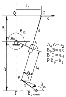
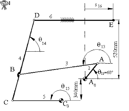
In order to show the application of Newton-Raphson method in mechanism analysis consider the mechanism shown. The closed form solution is not known. The loop closure equation in complex numbers yield:
|
 |
.
or in real numbers:

Which is a set of four equations in four unknowns in the form (input variable q12, is not considered as an unknown):
F1(q14, q15, s4) =0
F2(q14, q15, s4) =0
F3(q14, q15, s6) =0
F4(q14, q15) =0 =0
For a given value of input crank angle q12, we would like to solve the unknown position variables q14, q14, s4, s6. If q014, q015, s04, s06 are the initial estimates to the solution, q114, q115, s14, s16 are improved approximations and ds4= s14- s04 , ds6= s16- s06 ,dq14= q114- q014, dq15= q115- q015 are the difference between the two approximations, then this difference can be solved from equation (7) as:

or in real numbers:

Which are in the form:
![]()
Where A is the “coefficient matrix” in either complex or real form. E is the error in the loop closure equations with the initial estimates of the position variables (i.e. if the estimates are correct then E=0). The solution for the matrix equation is:
d=A-1E
After solving for the differences dq14 , dq15, ds4, ds5, the next improved condition is:
s(k+1)4=s(k)4+ ds4
s(k+1)5=s(k)5+ ds5
q(k+1)14=q(k)14+ dq14
q(k+1)15=q(k)15+ dq15
We repeat the steps until F(x(k+1))< ee , or (x(k+1)-x(k))< es. In mechanisms the solution usually converges within less then 10 steps if the initial guess is not too far away from the exact solution.
If the position analysis is to be performed for the whole cycle of the mechanism, one must make an initial guess for the dependent variables for the initial value of the crank angle and then solve for the correct values of the dependent variables using Newton-Raphson method. For the next position, when we increment the crank angle by a certain amount (usually less than 10 degrees), we can use the values of the position variables of the previous step as the initial guess of this step and perform the iterative method for this new position. If the step size is reasonably small, then the solution will converge to the next position of the mechanism. Since we are solving a nonlinear problem using stepwise linearization, if the step size is too large there is always the possibility of finding the solution for which the mechanism has to be assembled in a different configuration (i.e. if one has started with an open configuration the next solution may give a crossed configuration of the mechanism). Also, you may expect some numerical solution difficulties when the mechanism is at or near critical positions where the Jacobian matrix is zero or very small.
One can see that the method outlined is very general and can be applied for any planar mechanism that contains revolute, prismatic and cylinder-in-slot joints. If gear pairs are involved, the resulting linear equations can as well be inserted into the set of the loop equations. Furthermore a general computer program can be written to perform the kinematic analysis of any planar mechanism whose one position is known approximately.
Example
The six link mechanism shown is used as a rapier drive mechanism in textile industry. Link lengths are:
A0A=250 mm;
C0C= 600 mm;
CB = 350 mm;
BD= 600 mm;
A0C0= 710 mm;
AB=1225 mm and
DE= 1100 mm.
You are to determine s16 when q12=600.
As an initial guess for the position variables assume q13=2000;q15=1800; q14=800 and s16=400 mm when q12=600. We shall use MathCAD root finding routine, which utilises Newton-Raphson method (with some modifications). MathCAD output is as follows: You can see that when you write the loop equations and give the initial guess for the position variables, the Given and Find build in functions gives you the result in just a few steps while performing all the necessary iteration.
MathCAD FILE FOR EXAMPLE 2.8.
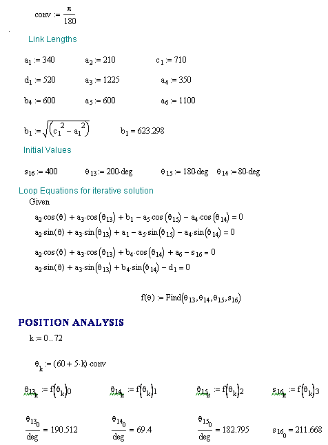
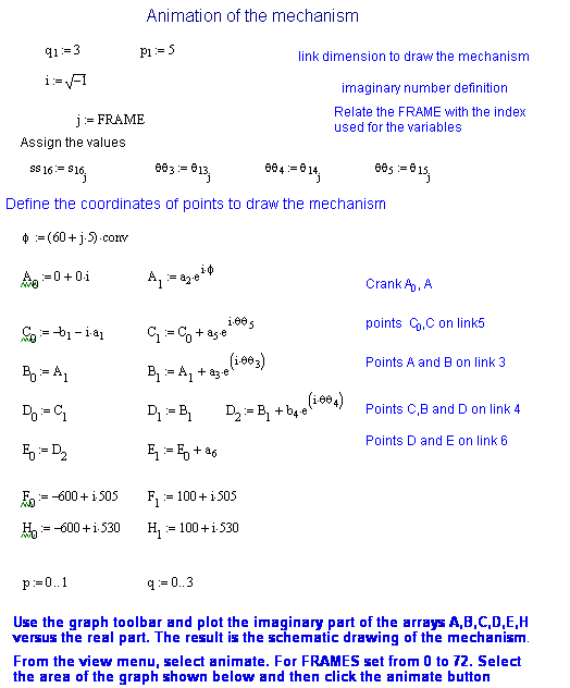
This iterative solution can also be solved in Excel as shown in the excel sheet below. After entering the link lengths we make an initial guess for the unknown position variables q13, q14, q15 and s16 for a given value of q12 in row 10 (A10 to E10) . Next, we write the x and y components of the two loop equations into cells F10 to I10. If our guess values were correct these values must be zero. It is not!! Now, let us square and add these values (errors) by typing "=F10^2+G10^2+H10^2+I10^2" into the cell J10. The value in this cell can only be zero if the values of the cells F10 to I10 are all equal to zero. Now we use the solver toolbox by clicking the "tools" and "solver". On the pop-up menu as the target cell we select J10 and for Equal To we select value of: 0. By changing Cells we select B10 to E10 as the initial guess. And then we click "solve" button on the pop-up menu. The values in cells B10 to E10 will change so that cell J10 is equal to zero, as seen on the next excel sheet

Fig. 2.50

Fig.2.51
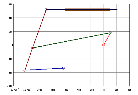
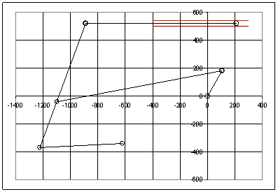
One can as well draw the mechanism by first determining the coordinates of the joints and then drawing lines between these coordinates in Excel chart As shown below
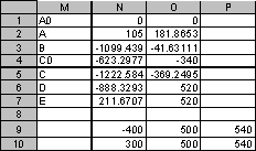
Fig. 2.52


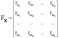 where Fkxmis the partial derivative of Fk with respect to xm.