8.3. BASIC CAM MOTION CURVES
In this section we shall discuss the basic philosophy in the selection of motion curves will be discussed and some well known motion curves will be explained. We shall consider the rise portion of the motion curve only. Later we shall see how a full motion curve can be constructed.
- Linear motion :
Equation describing a linear motion with respect to time is:
s= a1 t +a0
Assuming constant angular velocity for the input cam (w), since t =q/w :
s= a1q/w +a0
Let H= Total follower rise (Stroke)
b= angular rotation of the cam corresponding to the total rise of the follower.
Also assume when s = 0 q = 0 (rise is to start when t=0). With this assumption when s = H , q = b. when these boundary conditions are applied to the linear equation: a0=0 and a1=Hw/b. The linear motion curve is:
![]()
and
![]()
a = 0
The motion curve and velocity and acceleration curves are as shown. Note that the acceleration is zero for the entire motion (a=0) but is infinite at the ends. Due to infinite accelerations, high inertia forces will be created at the start and at the end even at moderate speeds. The cam profile will be discontinuous.
One basic rule in cam design is that this motion curve must be continuous and the first and second derivatives (corresponding to the velocity and acceleration of the follower) must be finite even at the transition points.
2. Simple Harmonic Motion (SHM):
Simple harmonic motion curve is widely used since it is simple to design. The curve is the projection of a circle about the cam rotation axis as shown in the figure. The equations relating the follower displacement velocity and acceleration to the cam rotation angle are:

In figure below the displacement, velocity and acceleration curves are shown. The maximum velocity and acceleration values given by equations:
vmax= ![]() , amax=
, amax= 
Note that even though the velocity and acceleration is finite, the maximum acceleration is discontinuous at the start and end of the rise period. Hence the third derivative, jerk, will be infinite at the start and end of the rise portion. This curve will not be suitable for high or moderate speeds.
In cases where the motion curve is composed of rise-return only, if the rise and return takes place for 1800 crank rotation each, simple harmonic motion curve results with a circular cam eccentrically pivoted (eccentricity = H/2, half the rise), as shown.

3. Parabolic or Constant Acceleration Motion Curve:
Noting that the velocity must be zero at the two ends, we can assume a constant acceleration for the first half and a constant deceleration in the second half of the cycle. The resulting motion curve will be two parabolas. This curve can be graphically drawn by dividing each half displacement into equal number of divisions corresponding to the divisions on the horizontal axis and joining these points with O and O’ for the first and second halves respectively. Point of intersection of these lines with the corresponding vertical lines yield points on the desired curve as shown
The equations relating the follower displacement, velocity and acceleration to the cam rotation angle are:
For the range 0 < q < b/2 For the range b/2 < q < b


![]()
![]()


In this case the velocity and accelerations will be finite. However the third derivative, jerk, will be infinite at the two ends as in the case of simple harmonic motion. Displacement, velocity and acceleration curves are as shown. This motion curve has the lowest possible acceleration.
In the literature, one can also find “skewed constant acceleration”, where the cam rotation angles for the acceleration and deceleration periods are not equal.
- Cycloidal Motion Curve:
If a circle rolls along a straight without slipping, a point on the circumference traces a curve that is called a cycloid This curve can be drawn by drawing a circle with center C on the line OO’. The circumference of the circle is equal to the total rise; or the diameter is H/p .The circumference is divided into a number of equal parts corresponding to the divisions along the horizontal axis. The points around the circle are first projected to the vertical centreline of the circle and then parallel to OO’ to the corresponding vertical line on the diagram (Fig. 8.18).
Figure 8.18
The equations relating the follower displacement, velocity and acceleration to the cam rotation angle are:
Within the curves we have thus far seen, cycloidal motion curve has the best dynamic characteristics. The acceleration is finite at all times and the starting and ending acceleration is zero. It will yield a cam mechanism with the lowest vibration, stress, noise and shock characteristics. Hence for high speed applications this motion curve is recommended. The maximum velocity and acceleration values are:

Compared to parabolic motion curve the maximum acceleration is 57% larger.
5. Straight line-Circular arc motion curve:
This curve is an improvement to the linear motion curve. To avoid infinite acceleration at the ends of the rise motion, circles are drawn as shown. Although the acceleration is finite, it will be of a high magnitude.
Using the figure it can be shown that (this is left as an exercise):
 ;
; ![]() H sinf ; q2=b-q1
H sinf ; q2=b-q1
Instead of circular arc the initial and final motions can be simple harmonic or constant acceleration as well as it will be shown in the following example. Straight line motion results in constant velocity. If we are to perform an operation such as cutting during the cam rise, constant velocity is the required motion characteristics.
Example 8.1.
The follower must then move by constant decelaration till it has a rise of 60 mm and dwell.
The rise motion is composed of three parts. Within the crank rotation 0<q<q1 we have constant acceleration (or parabolic) motion, within the range q1 < q < q2 we have constant velocity (or straight line) motion and within the range q2 < q < b we have constant deceleration (parabolic) motion curves. Angular velocity of the cam is given as w=50*p/30 = 5.238 s-1, therefore p/3 cam rotation will take place within Dt= 0.2 s. If the speed of the follower is kept at 200 mm/s during this phase of the motion, then the amount of rise with constant velocity is H’=200*0.2= 40mm. During the acceleration and deceleration periods total rise will be 20 mm. If we assume the rise for each constant acceleration periods is equal than there will be 10 mm rise for each interval. Note that the amount of crank rotation is not known for the constant acceleration periods.
Within the range 0 < q <q1 constant acceleration results with a second order motion curve ( a parabola). This curve can be written as:
s=c0+c1q+c2 q2
The boundary conditions is when q=0, s=0 and ![]() (since the motion starts from a dwell period, we want continuity on velocity); and when q=q1, s=10 mm and
(since the motion starts from a dwell period, we want continuity on velocity); and when q=q1, s=10 mm and ![]() Using the conditions for q=0 results c0=c1=0. The condition for q=q1 results with the equations:
Using the conditions for q=0 results c0=c1=0. The condition for q=q1 results with the equations:
c2q12 = H1 = 10mm
2c2q1w = 200mm/s
Solving the two equations we obtain: q1 = p/6 (=300 ) and c2=360/p2 .
For the deceleration period q2 < q < b again we have a second order algebraic curve s=c0+c1q+c2 q2 for the motion. When q = q2 = p/2 s=50 mm, ![]() ; and when q = b, s=H=60 mm and
; and when q = b, s=H=60 mm and ![]() . Using these boundary conditions
. Using these boundary conditions
| Db= b- q2 = p/6, | c0 = H- |
c1 = ![]() and c2 =
and c2 = ![]() . Now for the whole rise period the motion curves are:
. Now for the whole rise period the motion curves are:
Within 0< q <p/6 :
![]() ,
, ![]() mm/s and
mm/s and ![]()
Within p/6 < q <p/2
c0 = H-s=200 q , ![]() and
and ![]()
Within p/2<q <2p/3 :
![]() ,
, ![]() and
and ![]()
The displacement, velocity and acceleration curves are as shown. Note that although the displacement and velocity curves are continuous and the acceleration curve is finite, the third motion derivative (jerk) will be infinite at all the transition points. This motion curve can only be used for low speeds.
6. Trapezoidal Acceleration Curve:
Note that the Straight-line- circular arc curve was an improvement over the straight line motion curve since infinite acceleration was eliminated. Now let us consider constant acceleration motion curve. Although it had the lowest acceleration characteristics, the third derivative was infinite at the start, midpoint and at the end of the rise period since there was a step change on the acceleration curves. To obtain finite third order derivatives the steps in acceleration curve are changed to sloped lines, thus we obtain trapezoids for the acceleration curve as shown. Usually the uniformly accelerated portions of the curve is taken as 1/8 of the cam rotation angle for the total rise, b. In the remaining portions we have constant acceleration motion. Trapezoidal acceleration has the following characteristics.
a. It gives finite pulse, limited shock, wear, noise and vibration effects compared to the parabolic motion curve.
b. Compared to the third order motion curve (Cubic #1) or cycloidal motion curve, the peak acceleration is lower and the cam size is smaller.
c. For the same base circle radius, the transmission angle will be more favourable compared to the third order motion curve.
The curve can further be modified by eliminating the sharp corners of the trapezoids. For example at the ends and at the midpoint instead of uniform acceleration, one can use cycloidal or simple harmonic motion for 1/8 of the cam rotation angle. Trapezoidal motion curves (or modified trapezoidal) are suitable for high speed applications and are used especially in the automotive industry.
7. Cubic or Constant Pulse (#1):
Cubic #1 curve is the combination of two third order curves. There is no abrupt change at the start or the end of the cycle, but there is an infinite slope on the acceleration curve at the midpoint of the cycle, which is not advantageous. The curve is not very practical. The equations for the displacement velocity and acceleration are:
for 0 <q< b/2 for b/2 <q < b
![]()


![]()
![]()
![]()
The displacement, velocity and acceleration is plotted as shown.
8. Cubic or Constant Pulse #2 Motion Curve (2-3 polynomial curve):
The acceleration of cubic#2 curve is a continuous line with a negative slope. There is a finite acceleration at the ends which result with a step change. Jerk will be infinite at these points. Its characteristics is very similar to the harmonic motion curve. This curve is also known as 2-3 polynomial. The displacement, velocity and acceleration equations are :


9. Double Harmonic motion curve:
The curve is composed as the difference of two harmonics. It is an unsymmetrical curve. The rate of change of acceleration at the start of the rise period is small. It is best suited for D-R-R type of motion. The equations are
![]()
![]()

There are different methods used in generating motion curves satisfying the certain requirements. Note that for dwell-rise-return cams the main requirement is that there must be continuity of motion and its derivatives (velocity and acceleration). The displacement diagrams of the curves If we compare the displacement of the motion curves shown till now, one can see that there is very little difference . However when we compare the velocity and acceleration of these curves, large differences can be seen. Due to the difference in acceleration, dynamic characteristics will all be different.
In time, different ways of obtaining cam motion curves were devised. One way is the combination curve in which we use different simple functions within the rise period such as straight-line circular arc or trapezoidal motion curve. Another way of obtaining cam motion curve is to use higher harmonics (Fourier series), the third method is to use higher order polynomials and the fourth is the use of splines. All these methods have found use in cam design. Higher order harmonic motion curves, although they satisfy the boundary condition requirement, create vibration in the system. Therefore they are not preferred. We shall consider higher order polynomials and splines.
Figure 8.27

Figure 8.28
10. Polynomial Motion Curves:
The general expression for a polynomial is given by:
s= c0 + c1q + c2q2 + c3q3 +…….+cnqn
where
s= displacement of the follower,
q = cam rotation angle
ci = constants (i= 0,,,n)
n= order of the polynomial. For a polynomial of order n we have n+1 unknown constant coefficients. These constant can be determined by considering the end conditions. For cam motion we at least want to have continuity in displacement velocity and acceleration which results with the boundary conditions:,
for q=0 for q=b
s=0 s=H
![]()
![]()
![]()
![]()
Since there are 6 boundary conditions, one can evaluate the value of 6 constants Hence the polynomial must be of fifth order. The function and its derivatives are:
s= c0 + c1q + c2q2 + c3q3 + c4q4+c5q5
![]() c1 + 2c2q + 3c3q2 + 4c4q3+5c5q4
c1 + 2c2q + 3c3q2 + 4c4q3+5c5q4
![]() 2c2 + 6c3q + 12c4q2+20c5q3
2c2 + 6c3q + 12c4q2+20c5q3
Substituting the boundary conditions we have 6 equations in six unknowns (constants):
0= c0 (q=0, s=0)
H= c0 + c1 b + c2 b2 + c3 b3 +c4 b4+c5 b5 (q=b, s = 0)
0= c1 (q=0, ![]() )
)
0= c1 + 2c2 b + 3c3 b2 +4c4 b3 +5c5 b4 (q=b, ![]() )
)
0=2c2 (q=0, ![]() )
)
0=2 c2 + 6c3 b +12c4 b2 +20c5 b3 (q=b, ![]() )
)
Simultaneous solution of these equations yield:
c0=c1 =c2 =0
![]() ,
, ![]() ,
, ![]()
Hence, the fifth order polynomial is (This polynomial is commonly known as 3-4-5 polynomial) (Figure 8.30):


If we also ask for the third derivative to be zero at the ends (i.e. when q = 0 and when q = b: ![]() ) since there are 8 boundary conditions a seventh order polynomial will be required and we obtain 4-5-6-7 polynomial as:
) since there are 8 boundary conditions a seventh order polynomial will be required and we obtain 4-5-6-7 polynomial as:


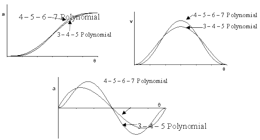
3-4-5 and 4-5-6-7 polynomials are compared in the above figure. Although 4-5-6-7 polynomial has zero jerk and finite fourth order characteristics. However, note that the maximum velocity and acceleration within the rise period has increased. This must also be taken into account.
Using the same procedure one can construct other higher order polynomials as well. However, one must not “overdesign”. Usually the difference between two high order motion curves is very small. If this difference is less that your manufacturing tolerances, even if you use a curve of very good acceleration and jerk characteristics, you will not be able to manufacture such a cam.
11. Spline Curves:
In the previous case we were able to fit a single polynomial for the rise. This procedure does not give us flexibility on the motion itself. In order to have some control over the motion the rise period is divided into a number of parts. The end points of these parts are called knots. The first and the last knot is the start and end of the rise and the boundary conditions must be satisfied. At the interior knots, in order to obtain continuity, the two adjacent polynomials must have the same value, slope (first derivative) and curvature (second derivative) etc. For each part a polynomial of order n is written. Using the boundary conditions at the knots the coefficients are solved. Since the mathematics involved is the topic on numerical analysis, this will be beyond the topic of this book.
Normalization of the motion curves
In order to compare the motion curves that were discussed we let:
w=1 rad/s
H= 1 unit
b= 1 radian
This procedure is known as “normalization”. Using this procedure one can then easily compare all these curves with respect to each other. This comparison is shown in Fig. 8.32 . Cv, Ca ve Cj, are the maximum velocity, acceleration and jerk values for the normalized curves. One can determine the maximum velocity, acceleration and jerk for any . H, w and b as:
![]()
Also the equations given for the normalized motion curves can be converted for any rise H, angular velocity w and crank rotation b by multiplying the equation by H substituting q/b instead of q. For example the cubic #2 curve is given as:

s=3q2+2q3
If we multiply the equation by H and substitute q/b instead of q we have:

Or:
![]()
Since Cv=1.5, Ca=6, the maximum velocity and acceleration values will be:
vmax=1.5*Hw/b , amax=6*H(w/b)2.
We have shown the motion curves for the rise and these curves start at q = 0 end at q = b with a rise s=H. The rise can start at any cam angle and we can have return motion. This can easily be performed by linear transformation of the motion curve. These transformations are shown below. For example in order to have a rise motion starting at an angle q=g, we must substitute (q-g) instead of q in any rise motion curve. In order to have a return starting at s=H at an angle q=g, any rise motion curve must first be subtracted from H and instead of q, (q-g) must be substituted (s= f(q)=H-s(q-g) will be the return curve starting at q=g and s=H). All motion curves except the double harmonic are symmetric motion curves.

Example 6.2.
Lay out the motion curve for a cam follower that is to have the following motion:
Rise 40 mm in 1200 crank rotation (cycloidal motion)
Dwell for 300 crank rotation,
Return 20 mm in 900 cam rotation (Simple harmonic motion),
Dwell for 300 crank rotation,
Return 20 mm in 600 cam rotation (parabolic motion),
The required motion curves as rise motion starting at q=00 will be given as:
Cycloidal Motion:
(H=40 mm, b=2p/3) ![]()
Simple Harmonic motion
| (H=20 mm, b=p/2) |
Parabolic Motion
| (H=20 mm, b=p/3) |  |
0 < q < p/6 |
 |
p/6<q < p/3 |
Now, let us transform these equations to the correct cam angles to obtain the equation s for 3600 cam shaft rotation:
| 0 < q <2p/3 | |
| 2p/3< q < 5p/6 | s = 40 |
| 5p/6< q < 4p/3 | |
| When simplified: | |
| 4p/3< q < 3p/2 | s=20 |
| 3p/2 < q < 5p/3 |  |
| 5p/3 < q < 11p/6 |  |
| When simplified: |  |
| 11p/6 < q < 2p | s=0 |
Using Excel the cam motion curve is drawn as shown in Figure 8.35. In Figure 8.34 the formula written excel cells are shown. In column A we enter cam angles from 0 (Cell A3) to 360 (cell A363) in degrees. In column B we convert these angles into degrees and in Column C, in rows 3 to 123 we have the formula for a cycloid, in rows 124 to 152 dwell at s=H= 40 mm etc.
In a similar fashion the derivative ds/dq and ![]() for the motion curves can be evaluated at every cam angle and the required formula can be entered into cells in Columns D and E respectively (w=1 s-1, constant). These curves are shown below.
for the motion curves can be evaluated at every cam angle and the required formula can be entered into cells in Columns D and E respectively (w=1 s-1, constant). These curves are shown below.
Depending on the application, manufacturing capabilities, etc. only one type of motion curve is usually used for both rise and return portions. In this example different curves are used just as an example.
![]()
![]()
![]()
![]() ©es
©es