CAM MECHANISMS

8.2. CAM DESIGN

Kinematic cam design is mainly concerned with the generation of the cam profile. From the standpoint of design, cams can be classified into two as:

Low-speed cams:For these cams the kinematics is our main concern. The inertia forces may be neglected. These cams exist in sewing machines in toys, in recording instruments. Since the surface quality is not very critical, these types of cams can be produced very cheaply (such as puncing from a sheet metal or molding plastics, etc). In certain applications they may even be used to reduce the number of parts in the mechanism. From the given kinematic requirements, the cam profile can be layed out without considering the dynamics of the system. However, one must keep in mind the smoothness of the cam surface and the pressure angle even for low speeds.

High-speed cams: Tthe concept of rigidity in case of high speeds will fail. In case of high speeds, low stiffness, large mass or resonance (all of which we shall call high speed cam). Dynamics of the system will be of great concern. For example, one of the application of cams is the internal combustion engine. The cam is used to open and close the intake and exhaust valves of the pistons. The motor speed of 6000 – 8000 rpm is very common. In such a case the follower must be raised (or the valve must be opened) in less than 0.05 seconds. Acceleration of the follower will reach several g’s.

Dynamic design of high speed cams is beyond the topic of this chapter. However, in performing the kinematic design one must take certain precautions, such as the limitation on the acceleration magnitude, so that the cam mechanism obtained can perform reasonably well at low or moderate speeds. For high speed cams certain restrictions must be placed to the input and output relation.

For low speed cams the motion curve which shows the input-output relation theoretically can be of any shape. Usually the motion repeats itself after a full rotation of the cam. Typical application is toys, automatic screw cutting machines, sewing machines, etc. When s = f(q) (0 < q < 2p) function is given. Even for low speed applications, this function must be continuous, and the slope of the curve must not be above a certain value. Otherwise, one may face problems such as excess power requirement, large forces at the bearings, etc. during the operation of the cam.

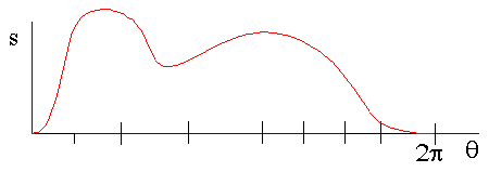
Figure 8.9

Figure 8.10.

In most cam applications the motion curve for the whole cycle is not exactly defined. What is usually required is in certain parts of the cam rotation the output must remain stationary. This condition is known as the dwell. For example, in internal combustion engines, we want a cam to keep the valve closed for a certain portion of the cycle (0 < q < b₁) and then open the valve as fast as possible and keep the valve open for some other portion of the cycle (b₂ < q < b₃). As another example consider a machine to form plastic cups. The die used to shape the cup must remain (dwell) at a low position so that the cup can be dispensed for a certain portion of the cycle (0 < q < b₁) and then it must move up to give the shape to the plastic and press it (usually heat is applied) open for some other portion of the cycle (b₂ < q < b₃)). The difference between the two applications is the amount of stroke s, the amount of force transmitted and the speed at which the two cams must rotate (In the first case it will be in the range of 3000 - 6000 rpm where as it will be around 30 to 60 rpm in the second example).

Usually the dwell periods must be kept as large as possible and the rise and return portions in between the dwells must be as fast as possible. However if the rise and return portion of the cycle is small, the displacement curve in between the two dwells will get steep hence the velocity and the acceleration will increase (assuming constant velocity of the input, the angular rotation of the cam, q, is proportional to the elapsed time). The cam motion curve can have the following global characteristics:

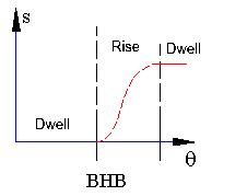
Dwell-Rise-Dwell (D-R-D): Afeter a certain dwell period the follower rises (or returns) to another dwell period. This is the most frequent cam motion. D-R-D portion of the cam cycle will be followed by a Dwell- Return-Dwell motion which is analysed in a similar manner with D-R-D (a)
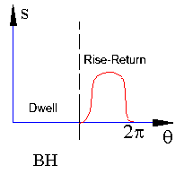
Dwell-Rise-Return (D-R-R): After a certain dwell period the follower rises and returns to the original motion (b)
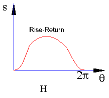
Rise-Return (R-R): There is no dwell period. For high speed applications one can in most cases instead of using cams one can use a slider-crank or any other mechanism with lower kinematic pairs (c)


(a)	(b)	(c)

Note that if the global characteristics of the motion curve is as shown in Fig 8.11 a and b, there will be no single function s(q) that defines the motion curve. Instead for each portion of the cycle we will have different functions.

For example for the dwell portions we will have s= 0 or s= H and . The motion curves for the rise and return portions has been selected as some basic mathematical functions so that the motion characteristics can be controlled.

CAM LAYOUT AND CAM NOMENCLATURE

Figure 8.7.

Let us explain the general procedure of graphical determination of the cam profile (generally known as cam lay-out) and explain the nomenclature used by a simple example. Assume a motion curve as shown in Fig. 8.7 is given. We would like to realize this motion curve using a radial cam with an inline translating roller follower. We must first determine the roller radius (rr) and the base circle radius (rb) onto which the cam profile will be applied. The roller radius is usually determined according to the allowable contact stress (known as Hertz stress) after we determine the forces acting at the contact point. The base circle radius is selected so that the cam profile is not very steep or in other words, the force transmission from the cam to the follower is reasonable. This will be explained in section 6.4. Let us assume that we know the roller radius (rr) and base circle radius (rb) Now, Let us draw a circle (prime circle) of radius rb+rr. The roller centre will be located on this circle when it is at a dwell at the bottom position. Now let us divide the motion curve and the prime circle at equal number of intervals. In figure 8.8 we have 12 equal intervals, corresponding 300 crank rotation each (in a real design case, especially for the rise and return portions, the number of intervals must be quite large to achieve a certain accuracy). In constructing the cam profile we perform kinematic inversion. We keep the cam fixed and release the fixed link and impart a motion to the fixed link such that the relative position of the links in this inverse motion is the same as the relative positions of the original motion. For example, assuming that the cam is rotating counter clockwise 300, the follower will be displaced by a distance s1 relative to the fixed link. When the cam is fixed, for the same relative motion, the fixed link will rotate by 300 clockwise relative to the cam (fixed) and the follower will be displaced by a distance s1 relative to the fixed link which has now rotated 300 clockwise. Hence we measure s1 radially from the prime circle. Thus we can determine the position of the centre of the roller on the follower and we can draw the roller circle for every increment. The cam profile is a smooth curve that is tangent to all these roller circles (Fig.8.8).