4.2 VELOCITY AND ACCELERATION ANALYSIS OF MECHANISMS-1
Velocity and acceleration analysis of mechanisms can be performed vectorially using the relative velocity and acceleration concept. Usually we start with the given values and work through the mechanism by way of series of points A, B, C, etc. Solving vector equations in the form:
VB = VA+ VB/A
VC= VB+ VC/B
etc. for velocity and
aB= aA+atB/A+anB/A
aC= aB+atC/B+anC/B
etc for acceleration. The points that one has to use are usually the revolute joint axes between the links since these are the points where the relative velocity or acceleration between the two coincident points on two different links are zero and they have equal velocity and accelerations. If we are to determine the velocity of a point on a link we must first determine the velocity of the points located at the joint axes.
![]() Another important consideration is that the acceleration analysis cannot be performed without performing the velocity analysis since the normal and Coriolis acceleration components can only be determined after the velocity analysis.
Another important consideration is that the acceleration analysis cannot be performed without performing the velocity analysis since the normal and Coriolis acceleration components can only be determined after the velocity analysis.
Loop equations can be used very effectively for velocity and acceleration analysis since the loop equations contain the necessary position variables. When the loop equations are differentiated with respect to time we obtain “velocity loop equations”. If the position variables are solved beforehand, these velocity loop equations will always yield a linear set of equations in terms of velocity variables which are the time rate of change of the position variables of the mechanism. When these velocity variables are solved for a given input condition, the velocity of any point on any link can be determined.
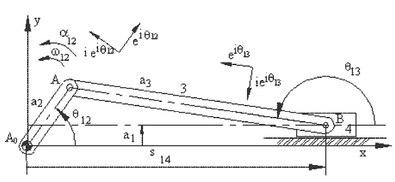
As a first example, consider a slider-crank mechanism shown above. We shall assume that q12 and its derivatives:
![]() are given. The loop closure and its complex conjugate is:
are given. The loop closure and its complex conjugate is:
![]() (1a)
(1a)
![]() (1b)
(1b)
For a given value of q12 we have seen how the position variable s14 and q13 can be solved. Differentiating the loop closure equation with respect to time we obtain the velocity loop equations as:
![]() (2a)
(2a)
![]() (2b)
(2b)
Where ![]() are the velocity variables. Note that the velocity loop equation is nothing but the vector equation:
are the velocity variables. Note that the velocity loop equation is nothing but the vector equation:
VB+ VA/B = VA
Physical explanation of the above equation is that point A is a permanently coincident point between links 2 and 3, since they are points on the revolute joint axis between these two links. Therefore VA2=VA3=VA. If we consider link 2, it is in a fixed axis of rotation and point A on link 2 has a velocity perpendicular to AA0 in the sense of w12 and its magnitude is w12 |AA0|. If we consider link 3, it is in a general plane motion. Points A and B are on this link. If we write the velocity of point A on link 3 using point B it is: VA3 =VB+VA/B = VA. . VA/B is perpendicular to AB. Point B is a permanently coincident point between links 3 and 4. Therefore VB3=VB4=VB. If we consider link 4, it is in a translation. Therefore the velocity of every point is tangent to the path, which is the slider axis. In the
velocity vector equation the unknowns are the magnitudes of VB and VA/B (which correspond to ![]() and
and ![]() in the velocity loop equation.
in the velocity loop equation.
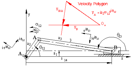
If the loop equations are to be solved graphically, unlike the analytical method where we group the unknowns on one side of the equality and the known values on the other side, we leave one unknown on both sides of the equation. The loop equation is rewritten as:
![]()
which is the vector equation:
VB = VA + VB/A
Note that
VB/A = - VA/B= ![]() .
.
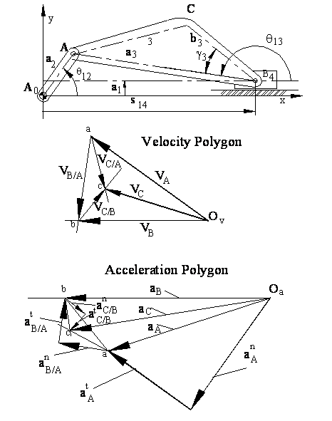
In order to determine the unknowns graphically, we first determine the magnitude of |VA|= w12|AA0|. Then using a certain scale factor, kv, a directed line (vector) whose magnitude is proportional to VA and direction of VA is drawn (seefigure below). From the starting point of this line, a line whose direction is that of VB, and from the tip a line whose direction is that of VB/A is drawn (VB is along the slider axis and VB/A is perpendicular to AB). The point of intersection gives us the tips of the vectors representing the velocities VB and VB/A . If we measure these lengths and then divide by the scale factor we have used for VA , the unknown magnitudes will be solved. The diagram thus obtained is known as the velocity polygon. For example if w13=dq13/dt is to be determined, first the length of the vector VB/A measured on the velocity polygon is divided by kv to determine the actual value of VB/A . Since VB/A = w13a3 and a3=|AB|, then w13=VB/A /a3. The direction of the angular velocity of link 3 is determined by the direction of VB/A . In the figure, since the velocity of point B relative to A (VB/A ) is downwards, in order to have this velocity at this position link 3 must have a clockwise angular velocity.
If the dependant position variables (s14 and q13) are to be solved analytically for a corresponding input position q12, the velocity loop equation will always give a linear relation between the velocity variables (w12, w13 and ![]() ). If the rate of change of the input variable (w12) is given, one can solve for the other two velocity variables w13) and
). If the rate of change of the input variable (w12) is given, one can solve for the other two velocity variables w13) and ![]() from the velocity equations by the methods of linear algebra. Since we have two equations (eq.2a and b) in two unknowns, we can apply Cramer’s rule:
from the velocity equations by the methods of linear algebra. Since we have two equations (eq.2a and b) in two unknowns, we can apply Cramer’s rule:
or
![]() (4)
(4)
and
 (5)
(5)
Note that one can as well obtain two scalar equations by equating the real and imaginary parts of the velocity loop equation and solve for the velocity variables as well. For the slider-crank mechanism these two scalar equations will be:
![]() (6)
(6)
and
![]() (7)
(7)
One will obtain exactly the same result from the solution of these two equations for the velocity variables w13 and ![]() .
.
For the acceleration analysis the velocity loop equations can be differentiated with respect to time to yield acceleration loop equations in terms of acceleration variables which are the second rate of change of the position variables. For the slider crank mechanism given, differentiating equations 2a and 2b with respect to time:
![]() (8a)
(8a)
![]() (8b)
(8b)
Where ![]() are the acceleration variables.. Note that this equation can be written as a vector equation in the form:
are the acceleration variables.. Note that this equation can be written as a vector equation in the form:
![]()
The acceleration loop equations are linear in terms of the acceleration variables (a12, a13 and ![]() ). If the input angular acceleration, a12 is known, these two equations can be solved for the unknowns a13 and
). If the input angular acceleration, a12 is known, these two equations can be solved for the unknowns a13 and ![]() using Cramer’s rule :
using Cramer’s rule :
 (9)
(9)
![]() (10)
(10)
Another approach is to differentiate the equations 4 and 5 directly to obtain acceleration variables. For example, differentiating equation 5, angular acceleration of link 3 will be obtained in the form:
 (11)
(11)
Although the terms may look different one will obtain the same result in either case.
Graphically, the acceleration loop equation can be solved by rewriting the acceleration vector loop equation as:
![]()
Where aB/A= - aA/B . The reason why the equation is written in this form is that we want to leave one unknown on each side of the equality. The magnitude of aB is one unknown and the magnitude of atB/A is the other unknown. Since the input angular velocity and acceleration are given atB/A and anB/A are known. If the velocity analysis is performed, magnitude of anB/A will be determined. We utilise a scale factor ka, to convert the acceleration vector magnitudes to a certain length. Starting with the vector atA or anA we draw the vectors atA , anB/A and anB/A of known magnitude and direction in an end-to-tip form as shown below. Then we draw a line in the direction of atB/A , which must be perpendicular to the line AB. The acceleration vector aB must be parallel to the slider axis. From the starting point we then draw a line parallel to the slider axis. The intersection of the two lines drawn will determine the magnitudes of aB andatB/A . The diagram thus obtained is known as the acceleration polygon. When we divide the measured magnitudes with the scale factor ka , we will obtain acceleration magnitudes.
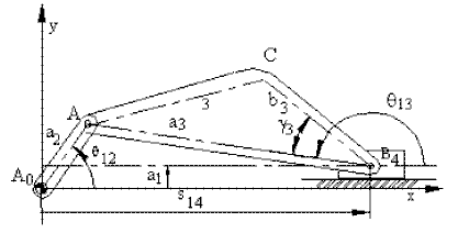
After obtaining the velocity and acceleration variables, one can determine the velocity and acceleration of any point C on the coupler link by writing its position vector in terms of position variables and differentiate the position vector to obtain the velocity and acceleration of point C. Referring to the figure above, The position vector rC is:
![]() (12)
(12)
Velocity and acceleration of point C is:
![]() (13)
(13)
![]() (14)
(14)
These equations are nothing but the vector equations:
VC=VB+VC/B
and
aC = aB + atC/B + anC/B
If one has solved the position (q13 and s14). velocity (w13 and ![]() ) and acceleration parameters (a13 and
) and acceleration parameters (a13 and ![]() ) for the given input condition (q12, w12 and a12), then note that all of the terms on the right hand side are known and one can determine the position, velocity and acceleration of point C.
) for the given input condition (q12, w12 and a12), then note that all of the terms on the right hand side are known and one can determine the position, velocity and acceleration of point C.
For the graphical solution, we can draw the vector equations for the velocity and acceleration of point C directly on the velocity and acceleration polygons drawn for the loop equations. Note that the velocity and acceleration of point C cannot be determined before solving the velocity and acceleration loop equations. From the tip of the vector VB, if we draw the velocity vector VC/B, the vector joining the starting point of VB to the tip of the vector VC/B will give us the velocity of point C. Similarly, The acceleration of point C can be determined by drawing the acceleration vectors anC/B and atC/Bstarting from the tip of the vector aB .The acceleration vector from the starting point of aB to the tip of the vector atC/B , will give us the acceleration of point C. Alternatively, note that the position of point C could have been written as:
![]() (15)
(15)
by differentiation:
![]() (16)
(16)
![]() (17)
(17)
Which are velocity and acceleration vector equations:
VC=VA+VC/A (18)
and
aC = atA + anA + atC/A + anC/A (19)
(15)
Let us label the tips of the vectors of the velocity and acceleration polygon by a lower case letter corresponding to the point whose velocity is represented (in case of acceleration the acceleration of point A and C are the sum of two or more acceleration vectors). The tips of the velocity vector VA,VB, VC and aA,aB, aC form triangles abc. We have an important theorem known as Mehmke's Theorem or "The principle of the velocity and acceleration image" :
The triangles abc formed on the velocity and acceleration polygons are similar to the triangle ABC of the mechanism link. The sense of abc is similar to the sense of ABC (if there is a counter clockwise rotation when going from A to B to C, there must be a counter clockwise rotation when moving from a to b to c on the velocity and acceleration polygons).
![]()
![]()
![]()
![]() ©es
©es